Policy-conditioned Models are More Generalizable

Ruifeng Chen^1,2, Xiong-Hui Chen^1,2, Yihao Sun¹, Siyuan Xiao¹, Minhui Li¹, Yang Yu^1,2

¹National Key Laboratory for Novel Software Technology, Nanjing University & School of Artificial Intelligence, Nanjing University, ²Polixir Technologies

Paper Code

Figure 1: An illustration of the difference between the development pipeline of policy-agnostic models (left) and policy-conditioned models (right). Suppose we wish to learn an environment where a biped robot is asked to move forward from an offline dataset including different locomotion patterns, such as jumping, walking, running, etc. Different locomotion patterns usually correspond to quite different transition patterns even though they can be regarded as a single task.

Abstract

In reinforcement learning, it is crucial to have an accurate environment dynamics model to evaluate different policies' value in downstream tasks like offline policy optimization and policy evaluation. However, the learned model is known to be inaccurate in predictions when evaluating target policies different from data-collection policies. In this work, we found that utilizing policy representation for model learning, called policy-conditioned model (PCM) learning, is useful to mitigate the problem, especially when the offline dataset is collected from diversified behavior policies. The reason beyond that is in this case, PCM becomes a meta-dynamics model that is trained to be aware of and focus on the evaluation policies that on-the-fly adjust the model to be suitable to the evaluation policies’ state-action distribution, thus improving the prediction accuracy. Based on that intuition, we propose an easy-to-implement yet effective algorithm of PCM for accurate model learning. We also give a theoretical analysis and experimental evidence to demonstrate the feasibility of reducing value gaps by adapting the dynamics model under different policies. Experiment results show that PCM outperforms the existing SOTA off-policy evaluation methods in the DOPE benchmark by a large margin, and derives significantly better policies in offline policy selection and model predictive control compared with the standard model learning method.

Video

10k-th iteration

30k-th iteration

50k-th iteration

We visualize the decision trajectories of MPC agents planned within the learned policy-conditioned models at different checkpoints during training (above), and the models' embedding visualization of trajectories with different performance (below). Notice that as the training progresses, the planning results achieve significantly better performance and the embedding distribution exhibits clustering tendency.

Method: Policy-conditioned Models

A. Value Gaps between True Dynamics and a Learned Model

The value gaps between true dynamcis $T^*$ and a learned model $\hat T$ is upper bounded by $$ |V^\pi_{T^*} - V^\pi_{\hat T}| \leq \frac{2\gamma R_{\max}}{(1-\gamma)^2}l(\textcolor{red}{\pi}, T^*, \hat T) $$ where $ l(\pi,T^*,\hat T)=\mathbb E_{s,a\sim\rho^\pi}D_{TV}(T^*(\cdot|s,a),\hat T(\cdot|s,a)) $ is the model error under the visitation distribution of the target policy $\pi$. This implies that as long as we reduce the model error under the target policy's distribution $\rho^\pi$, we can guarantee the reduce of the corresponding value gaps. However, since the target policy's visitation distirbution is not directly accessible, previous work (Janner 2019) further relaxes the bound to the model error under training distribution: $$ |V^\pi_{T^*} - V^\pi_{\hat T}| \leq \frac{2\gamma R_{\max}}{(1-\gamma)^2}l(\textcolor{red}{\mathcal D}, T^*, \hat T) +\frac{4R_{\max}}{(1-\gamma)^2}\sum_{i=1}^n w_i\max_s D_{TV}(\pi(\cdot|s),\mu_i(\cdot|s)) $$ where $ l(\pi,T^*,\hat T)=\mathbb E_{s,a\sim\mathcal D}D_{TV}(T^*(\cdot|s,a),\hat T(\cdot|s,a)) $ is the model error under the training data distribution $\mathcal D$, and the training data are collected by a set of behavior policies $\{\mu_i\}_{i=1}^n$, with corresponding propotion $w_i$. This intorduces additional policy divergence terms, irrevalent to the learned dynamics model, which just suggests minimizing the training training model error but ignores the dynamcis model's generalization to the target policies.
In contrast, we explicitly consider the dynamics model's generalization to different policies via a meta optimization formulation by conditioning the dynamics models on policies.

B. Policy-conditioned Model Learning

Conventional dynamcis model learning ignores the data source of each experience trajectory and directly learns a model from the mixed dataset, which we name Policy-agnoistic Models (PAM). Instead we propose to learn Policy-Conditioned Models (PCM) to adapt to different policies: $$ \hat F=\arg\min_{F\in\mathcal F}\sum_{i}w_i l(\mu_i,T^*,T_{F(\mu_i)}), $$ here $F$ is a policy-aware module mapping each policy to model parameters, optimized by minimizing the model error between true dyanmics $T^*$ and the models $T_{F(\mu_i)}$ conditioned on each behavior policy $\mu_i$ within the dataset.
In practice, we use a RNN-based encoder module $q_\phi$ to implement this policy-aware module, trained altoghter with the policy-conditioned model and a policy decoder: $$ \min_{\phi,\theta,\psi} \mathbb E_{t\sim[0,H-2],\tau^{(i)}_{0:t-1}\sim \mathcal D}[-\log T_\psi (s_{t+1}|s_t,a_t,q_\phi(\tau^{(j)}_{0:t-1}))-\lambda \mathcal R_\pi(q_\phi(\tau^{(j)}_{0:t-1}),\pi^{(j)},\theta)], $$ where $\mathcal R_{\pi}(q_\phi(\tau^{(j)}_{0:t-1}),\pi^{(j)},\theta)=\log p_\theta(a_t|s_t,q_\phi(\tau^{(j)}_{0:t-1}))$ is the policy reconstruction loss. The learned policy embeddings serve as contexts input into the policy-conditioned models together with the current state-action. During evaluation, PCM recognizes the target policy's embedding on the fly, and adapts model to make more accurate predictions on the target distribution. The overall development pipeline is illustrated in Figure 1.

C. Policy-conditioned Models have Lower Generalization Error

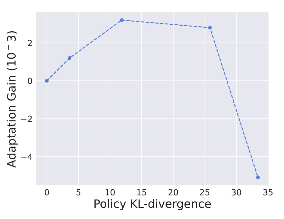
We show that the adaptation to policies reduces the PCMs' generalization error compared to conventional PAMs: $$ l(\pi,T^*,T_{\hat F(\pi)}) \leq \min_{\mu_i \in \Omega}\big\{\underbrace{l(\mu_i,T^*,T_{\hat F(\mu_i)})}_{\rm training~error} + \underbrace{L \cdot W_1(\rho^\pi, \rho^{\mu_i}) - C(\pi,\mu_i)}_{\rm generalization~error}\big\}, $$ where $L$ is the Lipschitz constant of the dynamics model w.r.t. the state-action inputs, and the adaptation gain term $C(\pi,\mu_i)$ is $$ C(\textcolor{blue}{\pi},\textcolor{red}{\mu_i}):=l(\textcolor{blue}{\pi},T^*,T_{\hat F(\textcolor{red}{\mu_i})}) - l(\textcolor{blue}{\pi},T^*,T_{\hat F(\textcolor{blue}{\pi})}). $$ This term summarizes the benefit brought by the policy adaptation effect, i.e., the reduced error of the target-policy-adapted model under the target distribution compared to that of the models trained under behavior policies.
We verify this adaptation gain empirically, showing positive gains within a resonable region around the dataset, which indicates the generalizability.

Figure 2. Illustrations of the adaptation gain of PCM for different unseen policies $\pi$, relative to a behavior policy $\mu_i$.

Experiments

A. Off-policy Evaluation (OPE)

To evaluate the performance of different policies, we can roll out the policy within the learned dynamics models to obtain simulated trajectories. We examine our PCMs in DOPE tasks and compare with sevaral OPE baselines, including model-free methods (FQE, DR, IS, DICE, and VPM) and model-based method using PAMs. The performance is measured by three indicators, i.e., Absolute error, Rank correlation, and Regret. The results show our PCM outperforms all the baselines with a large margin.

Figure 3. The performance of OPE in three metrics. To aggregate across tasks, we normalize the real policy values and evaluate policy values to range between 0 and 1. The error bars denote the standard errors among the tasks with three seeds.

B. Offline Policy Selection (OPS)

We train MOPO for 1000 epochs and record policy snapshots at the latest 20 epochs for OPS tasks. We use different OPE methods to evaluate these policies and select the best one among them. The table shows the normalized performance gains by different methods. It is noteworthy that the gains of FQE and PAM are even lower than directly selecting the last-epoch policy. In contrast, our approach shows a brilliant performance, implying that it reliably chooses a better policy for an offline RL algorithm to deploy.

Figure 4. Performance gain of offline policy selection for MOPO by different methods.

C. Model Predictive Control (MPC)

An accurate model can also be expected to perform effective model predictive control (MPC). We therefore compare our proposed PCM against PAM and the true dynamics. We use the cross-entropy method (CEM) as the optimization technique in MPC, which samples actions form a distribution closer to previous action samples yielding high rewards. Figure shows the cumulative rewards of the three methods during an episode, from which we can see that PCM performs similarly to the true dynamics and significantly outperforms PAM. We track several planning processes and compute regret $\sum_{i=t}^{t+T}\mathbb E_{T^*}[r(s_i,a_i^*)]-\sum_{i=t}^{t+T}\mathbb E_{T^*}[r(s_i,\hat a_i)]$ for both PAM and PCM, where $\hat a_{t:t+T}$ and $a^*_{t:t+T}$ are the optimal action sequences selected by the learned model and true dynamics respectively. PCM has lower regret than PAM, meaning that our approach tends to pick out actions that are closer to the optimal policy.

Figure 5. Performance and regret of MPC in HalfCheetah task. Left shows cumulative rewards within an episode in HalfCheetah. Right shows regrets of PAM and PCM during CEM, obtained by tracking several planning processes.

D. Analysis of Learned Policy Representation

We conduct a study to verify whether the PCM can learn reasonable policy representations. We select several policies with different performance and feed the trajectories generated by these policies into the policy encoder module of PCM. We visualize the outputted policy representations via the t-SNE (van der Maaten 2008) technique in Fig. 6(a). We find that the policies with similar performance have similar policy representations since there is a degree of resemblance between their performed actions, while the representations of policies with widely different performance are far apart due to their quite different behavior. In contrast, the representations without the policy reconstruction loss are randomly distributed. This result demonstrates that PCM can effectively identify similar policies and distinguish different policies.

Figure 6. Visualization for policy representations of different policies learned by PCM in HalfCheetah. Points are colored according to the normalized value.

BibTeX

@inproceedings{
      policyconditionedmodels,
      title={Policy-conditioned Environment Models are More Generalizable},
      author={Ruifeng Chen and Xiong-Hui Chen and Yihao Sun and Siyuan Xiao and Minhui Li and Yang Yu},
      booktitle={Forty-first International Conference on Machine Learning},
      year={2024},
      url={https://openreview.net/forum?id=g9mYBdooPA}
      }